KV and KV Caching in Transformers

Self Attention is the important technique that makes Tranformers great. It allows the model to pay attention to different parts of the input sequence as it generates next token. It transform each input token into context vector, which combines the information from all the inputs in given text. KV caching is only present for decoder only models like GPT or decoder part of encoder-decoder models.

Context vector calculation involves three components – query, key and value.

We will look into details on how it is computed.

Lets first look into how we could load GPT2 in our system and then use that example to understand KV and KV Caching.

One interesting topic would be understanding the KV caching and understanding how privacy could impact it.

Self-attention is achieved by transforming input sequence into three vectors – query Q, Keys K and Values V. Attention mechanism calculated weighted sum of the values based on similarity between query and key vectors, which along with original input passed through feed forward NN produces the final result.

Loading GPT2 model

from transformers import GPT2Tokenizer, GPT2LMHeadModel
tokenizer = GPT2Tokenizer.from_pretrained('gpt2')
model = GPT2LMHeadModel.from_pretrained('gpt2')

text = "She eats apple"
encoded_input = tokenizer(text, return_tensors='pt')
output = model.generate(encoded_input['input_ids'], max_length=10, num_return_sequences=2, num_beams=2, do_sample=False, temperature=0.0, pad_token_id=tokenizer.eos_token_id)

for i, sample in enumerate(output):
    decoded_text = tokenizer.decode(sample, skip_special_tokens=True)
    print(f"Sample {i + 1}: {decoded_text}\n")

This will generate two different samples of predicted text from GPT2 model. Sample 1 and Sample 2.

Sample 1: She eats apple pie, but he's not a

Sample 2: She eats apple pie, and I'm not sure

We can see the next text generated after “She eats apple” is “pie” we will look into how it could be calculated.

The important part in the generation process that we need to focus on is temperature=0.0, which means it will generate the same thing every time without providing probablistic result each time ie. the result will be deterministic to say. There are other ways to do it as well setting the seed as a static value, however this could be easier for now.

To understand the working of how model generated next tokens, we will have to get into the workings of various layers in the model. To do so we will have to return the attentions weights for the input texts to the model. Since generate() function only focuses on using the model to generate next prediction of tokens and not return those attention weights, we will be focusing on the forward passes method directly of the model instead.

# Forward pass on model including attentions
output = model(**encoded_input, output_attentions=True)

# attention weight - one tensor per layer
attentions = output.attentions

# attention tensor shape: (batch_size, num_heads, seq_length, seq_length)
# For simplicity, let's print the first attention layer and the first head
for layer_num, layer_attention in enumerate(attentions):
    print(f"Layer {layer_num + 1} Attention:")
    # layer_attention is of shape (batch_size, num_heads, seq_length, seq_length)
    # Get the attention values for the first head
    attention_head = layer_attention[0, 0, :, :].detach().numpy()
    print(attention_head)
    print()

Response:

Layer 1 Attention:
[[1.         0.         0.        ]
 [0.49838904 0.50161093 0.        ]
 [0.5619331  0.2192737  0.21879314]]

Layer 2 Attention:
[[1.         0.         0.        ]
 [0.971274   0.02872605 0.        ]
 [0.7161569  0.2259583  0.0578848 ]]
...

Layer 12 Attention:
[[1.         0.         0.        ]
 [0.6830764  0.31692368 0.        ]
 [0.8286772  0.09263436 0.07868845]]

Key points of self attention weights

• Query Q, Key K and Value V are all computed for the input embeddings
• each layer has its own weight matrices for Q, K and V vectors
• each attention head in multi-head attention mechanism has its own set of wieght matrics for Q, k and V.

In self-attention, we do matrix multiplication of the input vectors with weight matrices for Q, K and V ie. W_q, W_k and W_v which are computed during training process. This gives three vectors for input vector – Key Vector, Query Vector and Value vector which collectively is called Context Vectors.

Query Vector Q = x . W_q

Key Vector K = x . W_k

Value Vector V = x . W_v

Values for W_q, W_k and W_v can be retrieved for a model like GPT2 as below

layer_number = 0 
transformer_block = model.transformer.h[layer_number]
attention_layer = transformer_block.attn
computation_qkv = attention_layer.c_attn # c_attn is a linear layer responsible for generating Q, K and V

weights = computation_qkv.weight 
bias = computation_qkv.bias

W_q = weights[:model.config.n_embd, :]
W_k = weights[model.config.n_embd:2*model.config.n_embd, :]
W_v = weights[2*model.config.n_embd:, :]

print(f"Shape of W_q: {W_q.shape}")
print(f"Shape of W_k: {W_k.shape}")
print(f"Shape of W_v: {W_v.shape}")

Response:

Shape of W_q: torch.Size([768, 2304])
Shape of W_k: torch.Size([0, 2304])
Shape of W_v: torch.Size([0, 2304])

In first forward pass, there are single input token (in the example – “She”) that results in single value from multiplying the matrices for Key vector, and Query vector.

Q x K^T = QK^T

which then is multiplied with Value Vector to generate attention matrix.

The size of the matrix,

Q = [seq length , embeddings size]

K = [seq length, embeddings size] and KT = [embeddings size, seq length]

We can get the embedding shape in the layers for the model for GPT2 as belows

# Extract hidden states (embeddings)
# The last element in hidden_states corresponds to the output of the last layer
hidden_states = output.hidden_states
embeddings = hidden_states[-1]  # Last hidden state
print(embeddings.shape)

Response:

torch.Size([1, 3, 768])

Here, the tuple is defined in (batch_size, sequence length, hidden size). Batch size means, input of the model consists of single sequence, Sequence length is number of tokens in the input sequence and Hidden Size is the number of dimensions in the vectors that represent the tokens in model or size of hidden states and internal layers of the model (usually for similicity of the model, hidden size = embedding layer, and avoids additional transformations when using embeddings as input to transformer layers) .

For first input token,

emb_size = 768

Q [1, 768] x KT[768, 1] = QKT[1,1]

Then,

QKT[1,1] x V[1, 768] = Attention [1, 768]

Example:

[1,2,3] x [[4],[5],[6]]  = [32]

The same steps is done for multiple time for each tokens like for “She” to “eats”.

For second input token,

emb_size = 768

Q [2, 768] x KT[768, 2] = QKT[2,2]

Then,

QKT[2,2] x V[2, 768] = Attention [2, 768]

Example:

if emb_size = 3,

[1, 2, 3] x [1, 4] = [14, 32]
[4, 5, 6]   [2, 5]   [32, 77]
            [3, 6]        

In the similar way,for third token “apple”,

For second input token,

emb_size = 768

Q [3, 768] x KT[768, 3] = QKT[3,3]

Then,

QKT[3,3] x V[3, 768] = Attention [3, 768]

Example:

[1, 2, 3]   [1, 4, 7]   [ 14,  32,  50]
[4, 5, 6] x [2, 5, 8] = [ 32,  77, 122]
[7, 8, 9]   [3, 6, 9]   [ 50, 122, 194]

In this calculation process of attention in all individual tokens, also involves computation of attention of previous token. This is where caching of KV optimizes the process.

Looking at above figures , you can clearly see,

q1k1 computation is same for 1st, 2nd and 3rd token.

similarly, q1k1, q1k2, q2k1, q2k2 is same for 2nd and 3rd token computation of attention.

Each token has these common operations, that can be cached to speedup the computation.

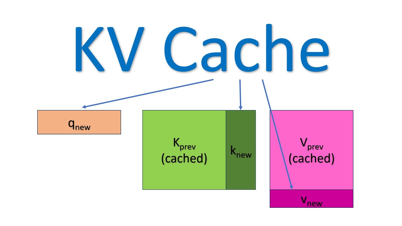
Following animation shows clearly on how it works.

(Fig: Animation of computation of attention involving caching [Ref])