Implementation of Differential Privacy (Part 1)

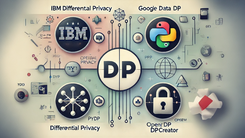
There are various differentially private algorithms to support Differential Privacy.

Bounded Mean, Bounded Sum, Laplace Mechanism, Exponential Mechanism, Private Histogram, Secured Multi Party Computation (Secured MPC), Differentially Private SGD, etc.

Of these algorithms Secured MPC, is one that I have worked in multiple other projects within domain of cryptography and blockchain as well. For the interest of privacy within ML models we will go through Differentially Private SGD in detail as well. We will be using libraries to approach the implementation within our applications.

Lets go with few concepts on DP like Function Sensitivity, Privacy Loss, Privacy Budget, etc.

Function Sensitivity – signifies how sensitive a function is to changes. The max change in the output of function when single individual’s data in input dataset is altered.

Privacy Loss – extend to which addition or removal of single individual’s data in dataset can influence the output of the query or computation

Privacy Budget – ϵ | epsilon – total privacy spending allowed while maintaining acceptable privacy guarantees

Following Openmined from the very early days when it was founded, I was very fond of understanding how ML and blockchain comes together – Decentralized AI. Other companies like SingularityNet were there however Openmined was more interesting to me. Openmined combines Federated learning with Homomorphic Encryption HME and blockchain to enable collaborative model to implement machine learning application in decentralized fashion.

Libraries on DP:

• IBM Differential Privacy ( diffprivlib )
• Google Differential Privacy
• Openmined DP (pydp)
• Opendp dpcreator

We will go through multiple libraries for implementation of DP, starting with IBM Differential privacy – which I think is very straight forward and simple implementation.

IBM Differential Privacy

Installation

$ pip install diffprivlib

Differential Privacy library has its own implementation of various ML algorithms, that does the training and is served for prediction. Lets go through how the library could be used for simple linear regression example. There are other examples as well that could be found in official repo – diffprivlib notebook.

Lets look into simple linear regression implementation using sklearn’s library.

Setting up dataset for running linear regression with diabetes dataset.

from sklearn import datasets
from sklearn.model_selection import train_test_split

dataset = datasets.load_diabetes()
X_train, X_test, y_train, y_test = train_test_split(dataset.data[:, :2], dataset.target, test_size=0.2)
print("Train #: %d, Test #: %d"% (X_train.shape[0], X_test.shape[0]))

Lets run default linear regression model from sklearn.

from sklearn.linear_model import LinearRegression
linear_regression = LinearRegression()
linear_regression.fit(X_train, y_train)
score = linear_regression.score(X_test, y_test)
print("R2 Score: %f"% score)

Response:

R2 Score: 0.069984

This models the linear regression using sklearn library. The result will remain the same for the same dataset used to train the regression model.

We will take a baseline for the model trained for evaluation

baseline = linear_regression.score(X_test, y_test)

Now running the differential privacy library,

from diffprivlib.models import LinearRegression

prv_linear_regression = LinearRegression()
prv_linear_regression.fit(X_train, y_train)
prv_score = prv_linear_regression.score(X_test, y_test)
print("epsilon=%f, R2 Score: %f" % (prv_linear_regression.epsilon, prv_linear_regression.score(X_test, y_test)))

Response:

epsilon=1.000000, R2 Score: -0.182144

Here the result changes everytime you fit the model, a different model is generated due to the randomness of Differential privacy. The r2 score changes everytime new model is used.

Lets understand the impact of privacy on model utility, to do that we will evaluate model score with privacy budget (ϵ). We will check the epsilon range from 10^-2 to 10². Lower value means strict privacy but lower model utility, and vice versa.

import numpy as np

epsilons = np.logspace(-1, 2, 100)
accuracy = []

for epsilon in epsilons:
    regr = LinearRegression(epsilon=epsilon)
    regr.fit(X_train, y_train)
    
    accuracy.append(regr.score(X_test, y_test))

import matplotlib.pyplot as plt

plt.figure(figsize=(8, 6))
plt.semilogx(epsilons, accuracy, label="Differentially Private Linear Regression", zorder=10)
plt.semilogx(epsilons, baseline * np.ones_like(epsilons), dashes=[2, 2], label="Normal Regression Baseline", zorder=5)
plt.xlabel("Privacy Budget (ϵ)", fontsize=12)
plt.ylabel("R2 Score", fontsize=12)
plt.ylim(-5, 1.5)
plt.xlim(epsilons[0], epsilons[-1])

plt.axvline(x=1, color='gray', linestyle='--', label="Moderate Privacy")
plt.axvline(x=0.1, color='red', linestyle='--', label="High Privacy")
plt.axvline(x=10, color='green', linestyle='--', label="Low Privacy")
plt.text(0.15, -4, "High Privacy\nLow Utility", color='red', fontsize=10, ha='center')
plt.text(1.5, 1.0, "Moderate Privacy\nBalanced Utility", color='gray', fontsize=10, ha='center')
plt.text(50, 1.2, "Low Privacy\nHigh Utility", color='green', fontsize=10, ha='center')

plt.legend(loc=2)
plt.title("Privacy-Utility Tradeoff", fontsize=14)
plt.grid(True, which="both", linestyle="--", linewidth=0.5)
plt.show()

With this chart we can see the relationship between epsilon and model score.